Building a fragility index using factor analysis

TL;DR

The ITC Fragility Index turns a set of business-survey questions about insecurity, trust, and economic performance into a single 0–100 fragility score for each business. We use exploratory factor analysis (EFA) to uncover three underlying dimensions—Human Security, Social Cohesion, and Economic Performance—and then use confirmatory factor analysis (CFA) to test the resulting structure. The three pillars are standardized and combined to produce the final index. Along the way, we demonstrate a practical, reproducible approach to using factor analysis in R to turn a multidimensional survey into a theoretically grounded composite index.¹

Introduction

Fragility affects businesses through multiple channels, from insecurity and social tensions to disruptions in economic activity. Capturing these different dimensions in a single measure presents a simple but important question: how can we turn a collection of survey responses into a meaningful measure of business-level fragility?

This blog demonstrates the methodology behind the ITC Fragility Index, constructed for the International Trade Center (ITC) and their small and medium enterprise (SME) fragility research in the SME Competitiveness Outlook 2023 ( ITC 2023). Data were obtained from the ITC Business Fragility Survey: a national business-level questionnaire aimed at assessing how SMEs cope within fragile social and political environments. Rather than simply adding the survey responses together, we use factor analysis to identify the underlying dimensions in the data and determine how individual indicators group together. Further details on the Survey and the related indicators can be found below as well as in the associated project description.

The analysis identifies three pillars—Human Security, Social Cohesion, and Economic Performance. We use exploratory factor analysis (EFA) to uncover this structure and confirmatory factor analysis (CFA) to test it. The resulting pillars are then standardized and combined to produce a single fragility score for each business.

The remainder of the blog walks through this process in R, illustrating how factor analysis can provide a transparent and reproducible foundation for constructing a composite index. The next two sections describe the Survey data and the factor analysis methodology. We then implement the methodology using a synthetic dataset for diagnostics, EFA, validation, and index construction. The final section concludes.

Data

Below, we describe the ITC Fragility Survey and generate a sample survey based on question statistics from the original Survey.

Survey overview

The ITC Business Fragility Survey is a national firm-level survey aimed at assessing how companies cope within fragile contexts. It contains data from businesses from eight countries collected between 2018 and 2022. The set of companies is sourced from the ITC SME Competitiveness Survey (SMECS), which is typically carried out in partnership with domestic business support organizations. The survey contacted 2,561 businesses, of which only 1,107 provided complete responses.

The ITC Business Fragility Survey includes questions about firm characteristics such as size, sector, and trade status, as well as the age and gender of the manager. It includes questions about business growth in terms of revenue and employees, as well as ease of access to financial resources and human capital. Finally, it queries business experience with fragility – encompassing finance, permits, regulations, competition, corruption, crime, etc. – and the coping mechanisms adopted by companies. The table below summarizes the survey questions related to fragility that feed into the Index.

The Index is based on a subset of firms from eight countries for which full and comparable data are available. The sample includes firms of different size, sector, and region.² As shown below, one in two surveyed firms are in services, one third are in agriculture, and the remaining 15 percent are in manufacturing. Nineteen out of twenty companies in the sample are SMEs. Importantly, the sample is not representative in all countries, and response rates vary across countries and sectors.

Synthetic sample

The Survey dataset is proprietary, so we rely on a synthetic sample for this blog post.

The Survey is entirely composed of binary or ordinal survey data. Thus, as a pre-step with the original Survey dataset, we standardize all variables between 0 and 1 to prevent any one variable from having undue influence over the analysis.

We generate a synthetic sample of 1,000 observations using synthpop and its function syn().

set.seed(1010)

df.survey <- readRDS(here::here("itc_fragility.rds"))

df.synthetic <- 
  synthpop::syn(
    df.survey[setdiff(names(df.survey), "FRAGID")], 
    k=1000
  )$syn

df.fragility <- tibble::rowid_to_column(df.synthetic, var="ID")

Methodology

The Fragility Index is created using factor analysis. Broadly, factor analysis seeks to define the fundamental dimensions assumed to underlie a set of variables. It combines a theoretical understanding of the subject matter with statistical techniques to summarize manifest variables into a smaller set of latent factors while minimizing information loss ( Hair et al. 2010).

Factor analysis relies on a number of assumptions ( OECD 2008):

1. Theoretically grounded variables. Factor analysis is most useful when conceptually defined dimensions can be represented by derived factors; if none exist, the technique cannot create valid factors. The exclusion of relevant variables, or the inclusion of spurious ones, affects which factors are uncovered, so the initial variable set should be driven by theoretical considerations as far as practicable.
2. Ordinal or binary data is acceptable. Factor analysis technically calls for quantitative data with at least an interval scale. However, as noted by Kim and Mueller ( 1978), an ordinal scale – ordered data without measurable differences between categories – is justifiable if its categories do not seriously distort the underlying scaling. Binary data is likewise permissible if correlations between variables are moderate, typically below 0.7.
3. Correlation is the whole point. Factor analysis leverages correlations between variables. Low correlations may preclude the approach, while high correlations may indicate multicollinearity. No firm quantitative threshold exists, but a substantial number of values in the correlation matrix should exceed 0.3. Measurement errors are also assumed to be uncorrelated.
4. Outliers matter. As with most statistical techniques, outliers can affect results. Tests for influential cases should be run, with comparison analyses between samples with and without outliers used as a robustness check; in extreme cases, outliers should be removed prior to analysis.

Factor analysis typically proceeds according to a fairly standardised recipe. We begin by confirming assumptions (2) and (3) regarding correlations through a number of pre-analysis diagnostics. We follow this with an EFA to estimate the index structure. Then, we perform a post-analysis validation to confirm the robustness of the estimated structure and to address assumption (4) that outliers do not affect results. When satisfied, we finish by constructing the index.

Diagnostics

Because factor analysis relies on estimating many correlations at once, some will look “significant” purely by chance. A large sample is the best protection against overfitting. As a general rule, you want at least five observations for every variable ( Hair et al. 2010). Our generated sample comfortably clears that threshold.

m.fragility <- cor(df.fragility[l.vars$all])

df.corr <- m.fragility |>
  as.table() |>
  as.data.frame() |>
  dplyr::rename_with(.fn=toupper) |>
  dplyr::rename(CORR = FREQ) |>
  dplyr::filter(as.character(VAR1) < as.character(VAR2))

l.corr <- list(
  n_pairs   = nrow(df.corr),
  n_over_03 = sum(abs(df.corr$CORR) >= 0.3),
  n_over_07 = sum(abs(df.corr$CORR) >= 0.7)
)

Across the 300 distinct pairwise correlations, we want a healthy number sitting in the “Goldilocks” zone between 0.3 and 0.7: strong enough to justify factor analysis, but not so strong that variables are redundant with one another. Out of all pairwise correlations, 75 have values greater than 0.3, representing approximately 25 percent of the dataset. Only 1 correlation has a value above 0.7. This suggests that there are a substantial number of correlations in the “Goldilocks” region.

While the above provides some descriptive evidence of commonality within our dataset, two formal tests confirm the data is suitable. Bartlett’s test of sphericity checks whether the correlation matrix is statistically distinguishable from an identity matrix – that is, whether the variables are correlated at all – while the Kaiser-Meyer-Olkin (KMO) measure checks sampling adequacy, with values below 0.5 signaling that the variables share too little in common to proceed. Because Bartlett’s test is sensitive to sample size, it is best implemented alongside KMO ( Tabachnick and Fidell 2013). We use the psych package and the cortest.bartlett() and KMO() functions to implement the tests, respectively.

psych::cortest.bartlett(m.fragility, n = nrow(df.fragility))

## $chisq
## [1] 8024.596
## 
## $p.value
## [1] 0
## 
## $df
## [1] 300

psych::KMO(m.fragility)

## Kaiser-Meyer-Olkin factor adequacy
## Call: psych::KMO(r = m.fragility)
## Overall MSA =  0.87
## MSA for each item = 
##            ID     FRAG_C_02  FRAG_C_03_A1  FRAG_C_03_A2  FRAG_C_03_A3 
##          0.46          0.53          0.81          0.83          0.84 
##  FRAG_C_03_A4  FRAG_C_03_A5  FRAG_C_03_A6  FRAG_C_03_A7  FRAG_C_03_A8 
##          0.93          0.93          0.92          0.90          0.91 
##  FRAG_C_03_A9 FRAG_C_03_A10 FRAG_C_03_A11 FRAG_C_03_A12 FRAG_C_03_A13 
##          0.89          0.93          0.91          0.91          0.92 
## FRAG_C_03_A14     FRAG_C_04  FRAG_C_05_A1  FRAG_C_05_A2  FRAG_C_05_A3 
##          0.92          0.58          0.83          0.71          0.72 
##  FRAG_C_05_A4  FRAG_C_05_A5     FRAG_C_06     FRAG_C_07     FRAG_C_08 
##          0.87          0.81          0.70          0.77          0.76

A significant Bartlett’s test alongside a KMO comfortably above 0.5 gives the green light to proceed with factor analysis.

Exploratory Factor Analysis

We next perform an exploratory factor analysis (EFA) on the remaining variables to identify the underlying dimensions in the data.³

The analysis proceeds in three steps:

1. Estimate the factor matrix. We first estimate the factor loadings, which indicate the strength of the relationship between each variable and factor. Higher absolute loadings indicate a stronger association and help us interpret the meaning of each factor.
2. Rotate the factor solution. After determining the number of factors to retain, we rotate the factor matrix to obtain a simpler and more interpretable structure. Ideally, each variable loads strongly on one factor and weakly on the others. We use the commonly applied varimax rotation.⁴
3. Evaluate and refine the solution. We then examine the rotated factor matrix for variables with low loadings or substantial cross-loadings across factors. When these occur, we remove the most problematic variable and repeat the analysis. We continue until the remaining variables produce a clear and interpretable factor structure.

Initial extraction

We run an exploratory factor analysis using the psych::fa() function and all Survey variables. We apply principal-axis factoring and retain factors with an eigenvalue above one – the standard “latent root” stopping rule ( Hair et al. 2010; OECD 2008).

l.fa <- list(
  initial = psych::fa(df.fragility[l.vars$all],
                      nfactors = sum(eigen(m.fragility)$values > 1),
                      fm = "pa",
                      rotate = "none")
)

## Factor Analysis using method =  pa
## Call: psych::fa(r = df.fragility[l.vars$all], nfactors = sum(eigen(m.fragility)$values > 
##     1), rotate = "none", fm = "pa")
## Standardized loadings (pattern matrix) based upon correlation matrix
##                  PA1    PA2    PA3    PA4    PA5    PA6    PA7     h2    u2
## ID                                                             0.0721 0.928
## FRAG_C_02                                                      0.0841 0.916
## FRAG_C_03_A1   0.425         0.529                             0.5666 0.433
## FRAG_C_03_A2   0.538         0.459                             0.6155 0.384
## FRAG_C_03_A3   0.526         0.511                             0.6261 0.374
## FRAG_C_03_A4   0.634                                           0.4380 0.562
## FRAG_C_03_A5   0.631                                           0.4290 0.571
## FRAG_C_03_A6   0.570                                           0.4047 0.595
## FRAG_C_03_A7   0.477        -0.302                             0.3306 0.669
## FRAG_C_03_A8   0.650                                           0.5691 0.431
## FRAG_C_03_A9   0.646                0.451                      0.6566 0.343
## FRAG_C_03_A10  0.678                                           0.5637 0.436
## FRAG_C_03_A11  0.653                                           0.5327 0.467
## FRAG_C_03_A12  0.636                                           0.4955 0.504
## FRAG_C_03_A13  0.656                                           0.4739 0.526
## FRAG_C_03_A14  0.641                                           0.4991 0.501
## FRAG_C_04                                                      0.0303 0.970
## FRAG_C_05_A1          0.716                                    0.5913 0.409
## FRAG_C_05_A2          0.881                                    0.8813 0.119
## FRAG_C_05_A3          0.808                                    0.7435 0.257
## FRAG_C_05_A4          0.557                                    0.3336 0.666
## FRAG_C_05_A5          0.415               -0.381               0.4067 0.593
## FRAG_C_06                                                      0.1214 0.879
## FRAG_C_07                                         0.359        0.2984 0.702
## FRAG_C_08                    0.370                             0.2092 0.791
##                com
## ID            3.04
## FRAG_C_02     4.64
## FRAG_C_03_A1  2.80
## FRAG_C_03_A2  2.81
## FRAG_C_03_A3  2.64
## FRAG_C_03_A4  1.19
## FRAG_C_03_A5  1.16
## FRAG_C_03_A6  1.50
## FRAG_C_03_A7  1.82
## FRAG_C_03_A8  1.75
## FRAG_C_03_A9  2.00
## FRAG_C_03_A10 1.48
## FRAG_C_03_A11 1.52
## FRAG_C_03_A12 1.48
## FRAG_C_03_A13 1.21
## FRAG_C_03_A14 1.45
## FRAG_C_04     3.97
## FRAG_C_05_A1  1.32
## FRAG_C_05_A2  1.28
## FRAG_C_05_A3  1.29
## FRAG_C_05_A4  1.16
## FRAG_C_05_A5  2.98
## FRAG_C_06     4.99
## FRAG_C_07     3.99
## FRAG_C_08     2.16
## 
##                         PA1   PA2   PA3   PA4   PA5   PA6   PA7
## SS loadings           5.272 2.687 1.346 0.620 0.459 0.357 0.233
## Proportion Var        0.211 0.107 0.054 0.025 0.018 0.014 0.009
## Cumulative Var        0.211 0.318 0.372 0.397 0.415 0.430 0.439
## Proportion Explained  0.480 0.245 0.123 0.056 0.042 0.033 0.021
## Cumulative Proportion 0.480 0.725 0.848 0.904 0.946 0.979 1.000
## 
## Mean item complexity =  2.2
## Test of the hypothesis that 7 factors are sufficient.
## 
## df null model =  300  with the objective function =  8.107 with Chi Square =  8024.596
## df of  the model are 146  and the objective function was  0.371 
## 
## The root mean square of the residuals (RMSR) is  0.019 
## The df corrected root mean square of the residuals is  0.028 
## 
## The harmonic n.obs is  1000 with the empirical chi square  113.093  with prob <  0.98 
## The total n.obs was  1000  with Likelihood Chi Square =  365.203  with prob <  8.99e-21 
## 
## Tucker Lewis Index of factoring reliability =  0.9414
## RMSEA index =  0.0387  and the 90 % confidence intervals are  0.0338 0.0438
## BIC =  -643.33
## Fit based upon off diagonal values = 0.993
## Measures of factor score adequacy             
##                                                     PA1   PA2   PA3   PA4   PA5
## Correlation of (regression) scores with factors   0.958 0.953 0.867 0.764 0.708
## Multiple R square of scores with factors          0.917 0.909 0.752 0.584 0.501
## Minimum correlation of possible factor scores     0.835 0.818 0.504 0.168 0.002
##                                                      PA6    PA7
## Correlation of (regression) scores with factors    0.609  0.561
## Multiple R square of scores with factors           0.371  0.315
## Minimum correlation of possible factor scores     -0.258 -0.371

Working through the loadings and uniqueness values in the factor matrix, four variables stand out as poorly explained which we iteratively drop:

• contract enforcement (FRAG_C_04)
• outlook on the business’s future (FRAG_C_07)
• the role of ethnicity and political ties (FRAG_C_06)
• security spending (FRAG_C_02)

Each has weak loadings across every factor and high uniqueness, which indicates that they are poorly explained by the retained factors.

Rotation

In the final iteration of our analysis, we obtain the output below after dropping the four variables above and applying a varimax rotation. The varimax rotation, which minimizes cross-loadings without changing total variance explained, leaves most variables loading cleanly onto a single factor. Ultimately, the objective is to minimize the number of significant loadings on each row of the factor matrix.

l.vars$final <- setdiff(l.vars$all, c("FRAG_C_02", "FRAG_C_04", "FRAG_C_06", "FRAG_C_07"))

l.fa$rotated <- psych::fa(
  df.fragility[l.vars$final],
  nfactors = 3,
  fm = "pa",
  rotate = "varimax"
)

## Factor Analysis using method =  pa
## Call: psych::fa(r = df.fragility[l.vars$final], nfactors = 3, rotate = "varimax", 
##     fm = "pa")
## Standardized loadings (pattern matrix) based upon correlation matrix
##                  PA1    PA2    PA3      h2    u2  com
## ID                                 0.00813 0.992 1.86
## FRAG_C_03_A1                 0.633 0.44842 0.552 1.23
## FRAG_C_03_A2   0.349         0.675 0.58962 0.410 1.56
## FRAG_C_03_A3   0.318         0.698 0.59328 0.407 1.42
## FRAG_C_03_A4   0.573         0.314 0.42680 0.573 1.55
## FRAG_C_03_A5   0.621               0.41046 0.590 1.13
## FRAG_C_03_A6   0.543               0.32178 0.678 1.19
## FRAG_C_03_A7   0.557               0.32774 0.672 1.12
## FRAG_C_03_A8   0.632               0.41751 0.582 1.09
## FRAG_C_03_A9   0.557               0.37881 0.621 1.45
## FRAG_C_03_A10  0.694               0.49152 0.508 1.04
## FRAG_C_03_A11  0.696               0.48530 0.515 1.00
## FRAG_C_03_A12  0.655               0.43421 0.566 1.03
## FRAG_C_03_A13  0.619               0.43162 0.568 1.25
## FRAG_C_03_A14  0.688               0.47506 0.525 1.01
## FRAG_C_05_A1          0.709        0.53129 0.469 1.12
## FRAG_C_05_A2          0.890        0.79531 0.205 1.01
## FRAG_C_05_A3          0.832        0.69571 0.304 1.01
## FRAG_C_05_A4          0.567        0.32694 0.673 1.03
## FRAG_C_05_A5          0.417        0.21038 0.790 1.41
## FRAG_C_08                    0.351 0.13539 0.865 1.20
## 
##                         PA1   PA2   PA3
## SS loadings           4.607 2.567 1.761
## Proportion Var        0.219 0.122 0.084
## Cumulative Var        0.219 0.342 0.425
## Proportion Explained  0.516 0.287 0.197
## Cumulative Proportion 0.516 0.803 1.000
## 
## Mean item complexity =  1.2
## Test of the hypothesis that 3 factors are sufficient.
## 
## df null model =  210  with the objective function =  7.768 with Chi Square =  7699.249
## df of  the model are 150  and the objective function was  0.794 
## 
## The root mean square of the residuals (RMSR) is  0.036 
## The df corrected root mean square of the residuals is  0.042 
## 
## The harmonic n.obs is  1000 with the empirical chi square  270.538  with prob <  6.01e-09 
## The total n.obs was  1000  with Likelihood Chi Square =  785.77  with prob <  8.29e-87 
## 
## Tucker Lewis Index of factoring reliability =  0.8809
## RMSEA index =  0.0651  and the 90 % confidence intervals are  0.0607 0.0697
## BIC =  -250.393
## Fit based upon off diagonal values = 0.982
## Measures of factor score adequacy             
##                                                     PA1   PA2   PA3
## Correlation of (regression) scores with factors   0.934 0.943 0.865
## Multiple R square of scores with factors          0.872 0.889 0.748
## Minimum correlation of possible factor scores     0.745 0.778 0.496

The rotated factor matrix reveals a clear three-factor structure. Two items—relating to delivery to clients and clients not paying their bills—show some cross-loading, but both capture clearly economic phenomena. We therefore retain them with the other economic indicators rather than dropping them. This follows the general guidance that cross-loading items should normally be removed unless there is a theoretical justification for retaining them ( OECD 2008).

The number of factors to retain is ultimately a matter of judgement, with both quantitative and qualitative criteria recommended in the literature OECD ( 2008). Quantitatively, the most common rule is the latent root criterion, which retains factors with eigenvalues greater than one. All three retained factors meet this criterion, with eigenvalues of 4.607, 2.567, and 1.761.

Together, the three factors account for 44.2% of the total variance, with the first factor explaining 22%, the second 12%, and the third 8%. Among the common variance captured by the factor solution, these correspond to 52%, 29%, and 20%, respectively.

The quantitative evidence is supported by the substantive structure of the survey. The variables group naturally into the three dimensions anticipated when the survey was designed as in Table 1: human security, social cohesion, and economic performance. The emergence of these three factors therefore provides both statistical and conceptual support for the proposed structure.

Index structure

That gives us the finalized index structure:

Validation

A factor structure that holds only under one particular set of modeling choices is of limited value. We therefore subject our proposed three-pillar index to several robustness checks:

1. confirmatory factor analysis (CFA);
2. alternative rotation methods;
3. bootstrap resampling;
4. polychoric correlations;
5. random split-samples; and
6. outlier detection.

We perform the CFA and provide details for the others.

Confirmatory factor analysis

The most direct test is a confirmatory factor analysis (CFA). Rather than allowing the data to determine the factor structure, we specify the three pillars identified above—Human Security, Social Cohesion, and Economic Performance—and test how well this structure reproduces the observed relationships. We use the lavaan package and its cfa() function.

cfa_model <- '
  HumanSecurity        =~ FRAG_C_03_A5 + FRAG_C_03_A6 + FRAG_C_03_A7 + FRAG_C_03_A8 + FRAG_C_03_A9 +
                            FRAG_C_03_A10 + FRAG_C_03_A11 + FRAG_C_03_A12 + FRAG_C_03_A13 + FRAG_C_03_A14
  SocialCohesion       =~ FRAG_C_05_A1 + FRAG_C_05_A2 + FRAG_C_05_A3 + FRAG_C_05_A5 + FRAG_C_05_A5
  EconomicPerformance  =~ FRAG_C_03_A1 + FRAG_C_03_A2 + FRAG_C_03_A3 + FRAG_C_03_A4 + FRAG_C_08
'

l.fa$cfa <- lavaan::cfa(cfa_model, data = df.fragility[l.vars$final])

## lavaan 0.7-2 ended normally after 151 iterations
## 
##   Estimator                                         ML
##   Optimization method                           NLMINB
##   Number of model parameters                        41
## 
##   Number of observations                          1000
## 
## Model Test User Model:
##                                                       
##   Test statistic                              1100.007
##   Degrees of freedom                               149
##   P-value (Chi-square)                           0.000
## 
## Model Test Baseline Model:
## 
##   Test statistic                              7362.361
##   Degrees of freedom                               171
##   P-value                                        0.000
## 
## User Model versus Baseline Model:
## 
##   Comparative Fit Index (CFI)                    0.868
##   Tucker-Lewis Index (TLI)                       0.848
## 
## Loglikelihood and Information Criteria:
## 
##   Loglikelihood user model (H0)               3092.622
##   Loglikelihood unrestricted model (H1)       3642.626
##                                                       
##   Akaike (AIC)                               -6103.245
##   Bayesian (BIC)                             -5902.027
##   Sample-size adjusted Bayesian (SABIC)      -6032.245
## 
## Root Mean Square Error of Approximation:
## 
##   RMSEA                                          0.080
##   90 Percent confidence interval - lower         0.076
##   90 Percent confidence interval - upper         0.084
##   P-value H_0: RMSEA <= 0.050                    0.000
##   P-value H_0: RMSEA >= 0.080                    0.490
## 
## Standardized Root Mean Square Residual:
## 
##   SRMR                                           0.075
## 
## Goodness of Fit Index:
## 
##   Goodness of Fit Index (GFI)                    0.903
##   90 Percent confidence interval - lower         0.894
##   90 Percent confidence interval - upper         0.912
## 
## Parameter Estimates:
## 
##   Standard errors                             Standard
##   Information                                 Expected
##   Information saturated (h1) model          Structured
## 
## Latent Variables:
##                          Estimate  Std.Err  z-value  P(>|z|)   Std.lv  Std.all
##   HumanSecurity =~                                                            
##     FRAG_C_03_A5            1.000                               0.132    0.630
##     FRAG_C_03_A6            1.058    0.069   15.347    0.000    0.140    0.564
##     FRAG_C_03_A7            0.741    0.052   14.271    0.000    0.098    0.517
##     FRAG_C_03_A8            1.126    0.066   17.185    0.000    0.149    0.647
##     FRAG_C_03_A9            1.213    0.075   16.101    0.000    0.160    0.597
##     FRAG_C_03_A10           0.972    0.054   18.038    0.000    0.128    0.688
##     FRAG_C_03_A11           1.044    0.058   18.112    0.000    0.138    0.692
##     FRAG_C_03_A12           1.060    0.060   17.601    0.000    0.140    0.667
##     FRAG_C_03_A13           1.141    0.066   17.302    0.000    0.151    0.653
##     FRAG_C_03_A14           1.055    0.059   17.956    0.000    0.139    0.684
##   SocialCohesion =~                                                           
##     FRAG_C_05_A1            1.000                               0.183    0.660
##     FRAG_C_05_A2            1.498    0.065   23.059    0.000    0.274    0.930
##     FRAG_C_05_A3            1.372    0.059   23.107    0.000    0.251    0.866
##     FRAG_C_05_A5            0.478    0.048    9.868    0.000    0.087    0.333
##   EconomicPerformance =~                                                      
##     FRAG_C_03_A1            1.000                               0.193    0.652
##     FRAG_C_03_A2            1.171    0.061   19.081    0.000    0.226    0.800
##     FRAG_C_03_A3            1.117    0.061   18.236    0.000    0.215    0.731
##     FRAG_C_03_A4            0.719    0.047   15.159    0.000    0.138    0.575
##     FRAG_C_08               0.326    0.046    7.031    0.000    0.063    0.249
## 
## Covariances:
##                     Estimate  Std.Err  z-value  P(>|z|)   Std.lv  Std.all
##   HumanSecurity ~~                                                       
##     SocialCohesion     0.002    0.001    1.829    0.067    0.065    0.065
##     EconomcPrfrmnc     0.015    0.001   10.954    0.000    0.578    0.578
##   SocialCohesion ~~                                                      
##     EconomcPrfrmnc    -0.003    0.001   -2.193    0.028   -0.082   -0.082
## 
## Variances:
##                    Estimate  Std.Err  z-value  P(>|z|)   Std.lv  Std.all
##    .FRAG_C_03_A5      0.026    0.001   20.357    0.000    0.026    0.603
##    .FRAG_C_03_A6      0.042    0.002   20.949    0.000    0.042    0.682
##    .FRAG_C_03_A7      0.026    0.001   21.253    0.000    0.026    0.732
##    .FRAG_C_03_A8      0.031    0.002   20.171    0.000    0.031    0.581
##    .FRAG_C_03_A9      0.046    0.002   20.679    0.000    0.046    0.644
##    .FRAG_C_03_A10     0.018    0.001   19.620    0.000    0.018    0.526
##    .FRAG_C_03_A11     0.021    0.001   19.563    0.000    0.021    0.521
##    .FRAG_C_03_A12     0.024    0.001   19.924    0.000    0.024    0.555
##    .FRAG_C_03_A13     0.031    0.002   20.105    0.000    0.031    0.574
##    .FRAG_C_03_A14     0.022    0.001   19.681    0.000    0.022    0.532
##    .FRAG_C_05_A1      0.043    0.002   20.443    0.000    0.043    0.564
##    .FRAG_C_05_A2      0.012    0.002    6.225    0.000    0.012    0.135
##    .FRAG_C_05_A3      0.021    0.002   11.744    0.000    0.021    0.251
##    .FRAG_C_05_A5      0.061    0.003   22.084    0.000    0.061    0.889
##    .FRAG_C_03_A1      0.050    0.003   18.662    0.000    0.050    0.574
##    .FRAG_C_03_A2      0.029    0.002   13.434    0.000    0.029    0.360
##    .FRAG_C_03_A3      0.040    0.002   16.483    0.000    0.040    0.465
##    .FRAG_C_03_A4      0.039    0.002   19.935    0.000    0.039    0.670
##    .FRAG_C_08         0.060    0.003   22.043    0.000    0.060    0.938
##     HumanSecurity     0.017    0.002   10.533    0.000    1.000    1.000
##     SocialCohesion    0.033    0.003   11.294    0.000    1.000    1.000
##     EconomcPrfrmnc    0.037    0.004   10.552    0.000    1.000    1.000

The CFA provides strong evidence that the individual indicators are associated with their proposed factors: all factor loadings are statistically significant. Standardized loadings are generally substantial, particularly for Human Security and Social Cohesion. The weakest relationship is between Economic Performance and FRAG_C_08, whose standardized loading is 0.25, suggesting that this indicator contributes relatively little to the latent factor.

The overall fit is more mixed. The model produces an RMSEA of 0.085 and an SRMR of 0.080, while the CFI and TLI are 0.868 and 0.848, respectively. These values indicate that the three-factor model does not provide a perfect representation of the data, but they are consistent with a reasonably coherent structure given the exploratory nature of the index and the characteristics of the survey data. Importantly, the CFA broadly reproduces the factor structure identified by the EFA rather than revealing a fundamentally different organisation of the indicators.

Alternative rotations

Varimax is only one of many possible rotation methods. A useful robustness check would therefore be to re-estimate the EFA using orthogonal and oblique rotations. If similar factor groupings emerge across these specifications, this would suggest that the proposed structure is not an artifact of the particular rotation method used.

Bootstrap resampling

Bootstrapping could provide an additional check on the stability of the number of factors ( Jackson 1993). The EFA could be repeated on, for example, 1,000 samples drawn with replacement, recording the number of factors selected in each replication. Consistent identification of three factors would provide evidence that the factor count is not overly sensitive to the particular sample.

Polychoric correlations

The EFA currently relies on a Pearson correlation matrix, despite the Fragility Survey containing exclusively binary and ordinal variables. A useful alternative would be to repeat the analysis using polychoric correlations, which are better suited to categorical data ( Watkins 2022). Comparing the resulting loadings and factor assignments with the preferred solution would indicate whether the factor structure depends on the choice of correlation matrix. In R, this can be implemented using the psych package and its polychoric() and fa() functions.

Random split-sample

With a sufficiently large sample, another straightforward check would be to randomly divide the observations into two or more independent subsamples and repeat the EFA separately. Recovering a similar factor structure across subsamples would provide evidence that the results are not driven by a particular subset of respondents.

Outlier detection

Finally, the analysis could be tested for sensitivity to influential observations. One approach would be to identify unusual observations using a convex-hull-volume-based influence measure derived from each observation’s leverage in the variable space ( Chatterjee et al. 1991). The EFA could then be repeated after removing the most influential observations. Little change in the resulting factor structure would suggest that the index is not being driven by a small number of unusual cases.

Index Construction

With the structure confirmed, the last step is turning three latent pillars into one fragility score per firm.

First, we predict each firm’s value on each of the three pillars from the confirmatory factor model using lavan::lavPredict(), then rescale each pillar onto a 0-100 scale using a max-min transformation – flipped so that higher values always mean more fragile:

$$\bar{x}_{i}^{j} = \frac{\hat{x}_{i}^{j} - \max(\mathbf{x}^{j})}{\min(\mathbf{x}^{j}) - \max(\mathbf{x}^{j})} \cdot 100$$

where \(\hat{x}_{i}^{j}\) is firm \(i\)’s predicted value on pillar \(j\), and \(\mathbf{x}^{j}\) is the full set of predictions for that pillar.

The overall Fragility Index is then simply the average across the three standardized pillars:

$$X_{i} = \frac{1}{3}\sum\limits_{j=1}^{3} \bar{x}_{i}^{j}$$

normalise <- function(x) {
  (x - max(x, na.rm = TRUE)) / (min(x, na.rm = TRUE) - max(x, na.rm = TRUE)) * 100
}

df.fragility_idx <- l.fa$cfa |>
  lavaan::lavPredict() |>
  as.data.frame() |>
  dplyr::mutate(dplyr::across(dplyr::everything(), normalise)) |>
  dplyr::mutate(
    ID = df.fragility$ID,
    INDEX = (HumanSecurity + SocialCohesion + EconomicPerformance) / 3
  ) |>
  dplyr::relocate(ID)

The result is a single number per firm – higher for firms facing more insecurity, less trust in institutions, and worse economic effects from instability – that can be compared across firms, sectors, and countries.

We now present some summary stats and plot a histogram of the Index and its Pillars. The Index has a mean of around 31 with a standard deviation of ±15. As can be seen from its histogram, its mass is mainly below 50. This is sensible given that the Human Security and Economic Performance Pillars are both weighted towards zero. The Social Cohesion Pillar drives the higher mean for the Index as its mass is distruted around 50.

idx_order <- c("Fragility Index",
               "Human Security",
               "Social Cohesion",
               "Economic Performance")

df.fragility_stat <- df.fragility_idx |>
  tidyr::pivot_longer(cols=-ID, names_to="PILLAR", values_to="VAL") |>
  dplyr::mutate(PILLAR = stringr::str_replace(PILLAR, "(?<=[a-z])(?=[A-Z])", " "),
                PILLAR = ifelse(PILLAR=="INDEX", "Fragility Index", PILLAR),
                PILLAR = factor(PILLAR, levels=idx_order)) |>
  dplyr::group_by(PILLAR) |>
  dplyr::summarise(MEAN = mean(VAL, na.rm=TRUE),
                   SD = sd(VAL, na.rm=TRUE))

Code 💻

df.fragility_plot <- df.fragility_idx |>
  tidyr::pivot_longer(cols=-ID, names_to="PILLAR", values_to="VAL") |>
  dplyr::mutate(PILLAR = stringr::str_replace(PILLAR, "(?<=[a-z])(?=[A-Z])", " "),
                PILLAR = ifelse(PILLAR=="INDEX", "Fragility Index", PILLAR),
                PILLAR = factor(PILLAR, levels=idx_order))

Plot 📈

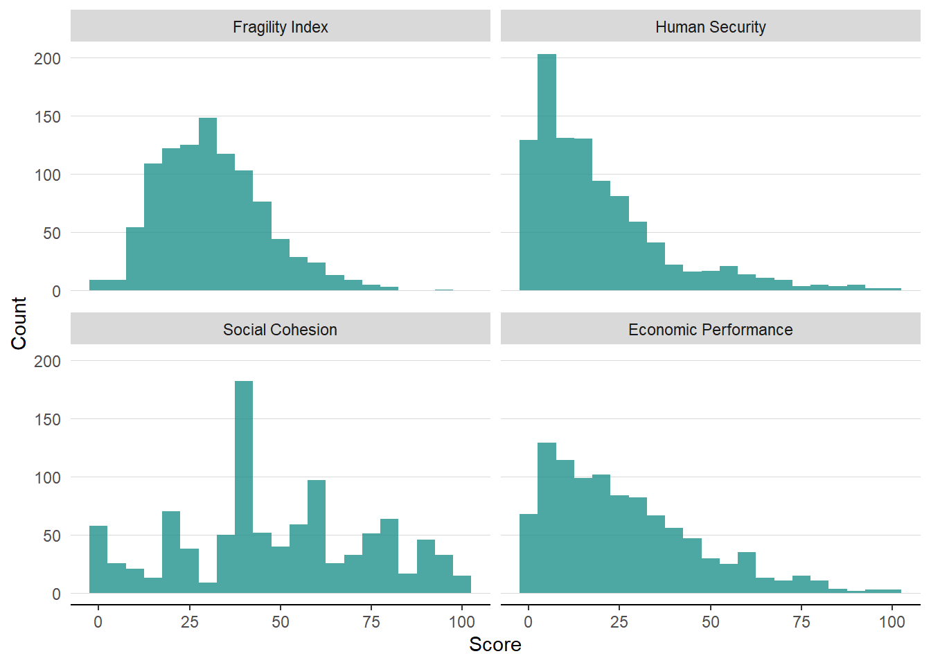
Figure 1: Fragility pillar and index histogram

Conclusion

The Fragility Index turns a multidimensional set of business-survey responses into a single, comparable 0–100 measure. EFA provides the link between the individual indicators and the three underlying pillars—Human Security, Social Cohesion, and Economic Performance—while CFA helps assess whether this structure is supported by the data. The methodology provides a transparent and reproducible approach to constructing composite indicators. The resulting Index and its Pillars can be used as standalone measures of fragility or incorporated as explanatory variables in broader analyses of local business outcomes.

References

Chatterjee, S, L Jamieson, and F Wiseman. 1991. “Identifying Most Influential Observations in Factor Analysis.” Marketing Science 10 (2): 145–60.
Hair, JF, WC Black, BJ Babin, and RE Anderson. 2010. Multivariate Data Analysis. Vol. 7. Pearson.
ITC. 2023. SME Competitiveness Outlook 2023: Small Businesses in Fragility: From Survival to Growth. International Trade Centre. https://www.intracen.org/resources/publications/sme-competitiveness-outlook-2023-small-businesses-in-fragility-from-survival.
Jackson, DA. 1993. “Stopping Rules in Principal Component Analysis: A Comparison of Heuristical and Statistical Approaches.” Ecology 74 (2): 2204–14.
Kim, J, and CW Mueller. 1978. Factor Analysis: Statistical Methods and Practical Issues. Paper Nos. 07-014. Sage University Paper Series on Quantitative Applications in the Social Sciences.
OECD. 2008. Handbook on Constructing Composite Indicators: Methodology and User Guide. Organization for Economic Cooperation; Development; and, Joint Research Centre, European Commission.
Tabachnick, BG, and LS Fidell. 2013. Using Multivariate Statistics. Vol. 6. Pearson.
Watkins, MW. 2022. A Step-by-Step Guide to Exploratory Factor Analysis with Stata. Routledge.
-
All analysis herein uses R, where the original analysis and Index were prepared in Stata. ↩︎
Firm sizes are defined by employee count: “Micro” 1 to 9; “Small” 10 to 49; “Medium” 50 to 249; and “Large” 250 or more. ↩︎
Note that there are two types of factor analysis: common and component. They have contrasting objectives where the former is used to identify latent dimensions represented in the data, while the latter is primarily a data reduction technique ( Hair et al. 2010). Here, we focus on common factor analysis. ↩︎
Rotation changes the individual factor loadings and eigenvalues, but not their sum. ↩︎